Notes of the seminar ‘On the slice rank of functions’

Last week, I gave a seminar on the slice rank of functions (probably one of many concerning that particular subject since last year). The motivation being mainly that I, together with my advisors Jan De Beule and Philippe Cara, wanted to understand this method better, so what better way to understand something than to talk about it with fellow mathematicians?

I want to write down some of the material I presented on the blackboard, primarily to have a reference and some notes for myself, but perhaps they can also give someone else a better understanding of the ideas and concepts regarding this topic. I have not seen the visual interpretation of the different notions of rank is anywhere else, so this might be interesting as well. Let me know if this has helped you or if something needs more explanation!

Background

Last year, the combinatorial world was stunned by a series of results by Croot-Lev-Pach, Ellenberg-Gijswijt regarding arithmetic progressions in certain groups. I will not try and give an complete account of these, as several sources around the web have done so already quite extensively (blog post by Anurag Bishnoi; a rendition of the proof by Doron Zeilberger and references on Gil Kalai’s blog). As an indicator of the gravity of these two results, both have been published in the Annals of Mathematics in the beginning of this year. Instead, I will try to elude the idea of ‘slice rank’ of a tensor, as was defined by Terry Tao in his reformulation of the Ellenberg-Gijswijt proof. I will try to indicate where the idea might have come from and how one can understand it in a sort of geometrical way. Most, if not all, of the theory can be developed for general tensors (see again Terry’s blog), but we will restrict ourselves to to a special case, which we will explain in the next paragraph. The reason for this is that I find the concepts easier to explain in this specific setting. So without further ado, let’s get on with it.

Functions of a finite set to a field

People comfortable with tensor products and know why an n-variable function $f : A_1 \times \dots \times A_n \rightarrow \mathbb{F}$ , where each $A_i$ is a finite set and $\mathbb{F}$ is a field, is a special case of a tensor, can skip this section.

For those who aren’t (like myself), here’s a short explanation why. Consider a finite set $A$ , a field $\mathbb{F}$ and the set of functions $A \rightarrow \mathbb{F}$ , denoted by $\mathbb{F}^A$ . For every element $a \in A$ , we can consider its characteristic function $\delta_a(x)$ , which is 1 if $x=a$ and 0 otherwise. Endowing the set $\mathbb{F}^A$ with an addition and multiplication with a scalar from $\mathbb{F}$ in the natural way, we see that $\mathbb{F}^A$ is isomorphic as a vector space to $\mathbb{F}^{|A|}$ , with a natural basis $\delta_a(x)$ , $a \in A$ .

Therefore, for two finite sets $A$ and $B$ , we can consider the tensor product $\mathbb{F}^A \otimes\mathbb{F}^B$ . One can check that this is a vector space isomorphic to $\mathbb{F}^{|A||B|} \cong \mathbb{F}^{A \times B}$ , which can be seen by the isomorphism $\delta_a(x) \otimes \delta_b(y) \leftrightarrow \delta_a(x)\delta_b(y)$ . This means for example that any function $f: A \times B \rightarrow \mathbb{F}$ can be expanded in the natural basis of delta functions as

$f(x,y) = \sum_{(a,b) \in A \times B}f(a,b)\delta_a(x)\delta_b(y).$

In the same way, one can write $f(x_1,\dots,x_n)$ as a sum of functions of the form $\delta_{a_1}(x_1) \otimes \dots \otimes \delta_{a_n}(x_n)$ , where $a_i \in A_i$ , and is therefore a tensor.

Tensor rank versus (multi-)slice rank

For most instances of ‘rank of an object’, we have the following heuristic rule:

object of rank k = sum of k objects of rank one (and not less)

Meaning that, in order to define a rank function, it suffices to specify the rank one objects. This is for example the case for the usual definition of tensor rank, and will also be the case for the other two rank functions we define. As previously remarked, we will only define these rank function for the special case of n-variable functions.

In order to avoid cumbersome notation, we use the following convention. Let $[n] = \{1,\dots,n\}$ and $I = \{i_1,\dots,i_k\} \subseteq [n]$ . Then by $X_I$ we mean $X_{i_1} \times \dots \times X_{i_k}$ and for a function $f: X_I \rightarrow \mathbb{F}$ we write $f(\vec{x}_I)$ instead of $f(x_{i_1},\dots,x_{i_k})$ .

A function $f(\vec{x}_{[n]}): X_{[n]} \rightarrow\mathbb{F}$ is of tensor rank one if and only if there exist functions $g_i:X_i \rightarrow\mathbb{F}, 1 \leq i \leq n$ such that $f(\vec{x}_{[n]}) = g_1(x_1)\dots g_n(x_n)$ . In a way, the function ‘splits’ completely.

A function $f(\vec{x}_{[n]}): X_{[n]} \rightarrow\mathbb{F}$ is of slice rank one if and only if there exists $i$ and functions $g:X_i \rightarrow\mathbb{F}, h:X_{[n]\backslash \{i\}}$ such that $f(x_{[n]}) = g(x_i)h(x_{[n]\backslash \{i\}})$ . In words: we can ‘slice off’ one variable from the function.

A function $f(\vec{x}_{[n]}): X_{[n]} \rightarrow\mathbb{F}$ is of multi-slice rank one if and only if there exists $I \subseteq [n]$ and functions $g:X_I \rightarrow\mathbb{F}, h:X_{[n] \backslash I}$ such that $f(x_{[n]}) = g(x_I)h(x_{[n] \backslash I})$ . Here we relax the notion of rank even more, by slicing off several variables at once.

Bounds and examples

Let $f: X^{[n]} \rightarrow \mathbb{F}$ be an n-variable function. The first inequality is immediate when comparing the definitions:

multi-slice rank( $f$ ) $\leq$ slice rank( $f$ ) $\leq$ tensor rank( $f$ ).

A decomposition of $f$ into a basis of delta functions shows that

slice rank( $f$ ) $\leq \min_i |X_i|,$

tensor rank( $f$ ) $\leq$ slice rank( $f$ ) $\cdot \max_i |X_i|,$

and if $g: X^{[n]} \rightarrow \mathbb{F}$ is another n-variable function then

multi-slice rank( $f \cdot g$ ) $\leq$ tensor rank( $f$ ) $\cdot$ slice rank( $g$ ).

These bounds can be found in the papers of Blasiak et. al and Naslund.

We can show some examples to see that tensor rank, slice rank and multi-slice rank may differ heavily. Let $X$ be a finite set, $X^k$ the k-fold Cartesian product of $X$ with itself and $\mathbb{F}$ a field.

Example 1. Consider the function $\delta(x,y):X^2 \rightarrow \mathbb{F}$ which is 1 if $x=y$ and 0 otherwise. Define $f(x,y,z): X^3 \rightarrow \mathbb{F}, f(x,y,z)=\delta(x,y)$ . This function has tensor rank $|X|$ and slice rank 1.

This example shows that the second inequality is sharp. The gap between slice rank and multi-slice rank can also be big, as shown in the next example.

Example 2. Define $f(x,y,z,w): X^4 \rightarrow \mathbb{F}, f(x,y,z,w)=\delta(x,y)\delta(z,w)$ . This function has slice rank $|X|$ and multi-slice rank 1.

Visually representing the differences

Clearly for $n=2$ , the three notions coincide, so we will consider the case $n=3$ to see the difference between tensor rank and (multi-)slice rank (in this case, the last two definitions of rank coincide). We will use a higher-dimensional version of the following fact: consider a function $f: A \times B \rightarrow \mathbb{F}$ and construct the matrix of values $M$ . Its rows are indexed by $A$ , its columns by $B$ and the $(a,b)$ -entry equals $f(a,b)$ . Then the following should be clear: $f$ has tensor rank (or (multi-)slice rank) 1 if and only if its matrix of values $M$ has matrix rank one.

When considering a function $f: A \times B \times C \rightarrow \mathbb{F}$ , we can construct a hypermatrix of values instead of a matrix, which should be seen as a 3D array of $|A||B||C|$ points. Here the notions of tensor rank and (multi-)slice are clearly not equivalent. For simplicity, suppose that $A = B = C = \{0,1\}$ , so we can draw the values of $f$ on the cube $\{0,1\}^3$ .

We can first consider the case when a function has tensor rank one. When drawing its associated hypermatrix with the values, we get the following picture.

Figure 1: The function has tensor rank one.

We see that in all three directions, we have ‘scalarity’ (by lack of a better word), by which I mean that (every value on) every hyperplane is a scalar multiple of (a value on) any parallel hyperplane. This clearly also holds if $A, B$ and $C$ are arbitrary finite sets. This is a quite strong condition, which seems natural to relax.

Suppose that the function has slice rank one, then the picture is the following.

Figure 2: The function has slice rank one.

Clearly, the property of scalarity of the hyperplanes in all directions / all parallel classes is now replaced by scalarity of hyperplanes in one direction, namely in the direction indexed by the set whose variable can be split off.

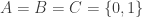
To understand the difference between slice rank and multi-slice rank, using this same idea of a hypermatrix of values, we would need to draw a 4D hypermatrix. We will make an attempt in doing so. We will again consider the simple case when all sets involved are $\{0,1\}$ . First we need to understand how one can draw a 4D cube in 2D.

A cube in 2D can be drawn as below: draw two squares, one sitting inside the other, and connect corresponding points of the squares.

cube in 2D

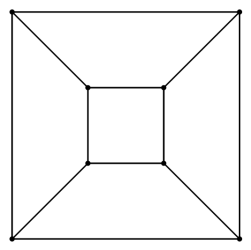
A 4D cube can be realised in 3D in the same way: take two cubes, one inside the other and connect corresponding points. However, this blog is as of now restricted to two dimensions (high hopes for the distant future!), so we need to draw these two cubes again the in plane. This can be done in the following way.

The blue and red cube are the original cubes, corresponding points are connected by the green lines.

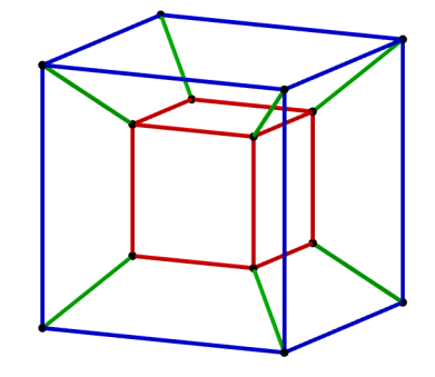
Using this visual representation, we can try to distinguish functions of slice rank one and of multi-slice rank one. First we start with a function of slice rank one and its hypercube of values.

slice rank on hypercube

As you can see, the red and blue cubes, contained in the hypercube, exhibit the scalarity phenomenon. This indeed means that we have scalarity of hyperplanes (which in this case are three-dimensional spaces on the hypercube, i.e. cubes) in one direction. In contrast, below is the hypercube of values for a function of multi-slice rank one.

multi-slice rank on hypercube

In this case, we have scalarity of the red and blue subspace, but in this case the subspaces are planes, as opposed to cubes. The pictured red and blue planes are not the only pair of planes related by scalarity, can you find more?

Applications to combinatorics

The definition of slice rank and multi-slice rank of an n-variable function are not pulled from thin air. They have appeared implicitly in the Croot-Lev-Pach and Ellenberg-Gijswijt paper and are roughly based on the following basic fact.

Fact. Consider a polynomial $P(x)$ one variable of degree $n$ . When we consider $P(x+y)$ and expand this into a sum of monomials $x^ky^l$ , we know that for every monomial either $k \leq n/2$ or $l \leq n/2$ .

This means that if we define a two variable function $Q(x,y)$ by $Q(x,y)=P(x+y)$ , one can bound the tensor rank of $Q(x,y)$ by twice the number of monomials $x^ky^l$ where $k \leq n/2$ . When considering three or more variables (e.g. $Q(x,y,z) = P(x+y+z)$ ), we need to replace tensor rank by slice rank.

This gives one half of an inequality. The other half comes from a generalization of the fact that the matrix rank of a diagonal matrix is the number of non-zero elements on its diagonal.

Lemma. Let ${k \geq 2}$ , let ${A}$ be a finite set, let $\mathbb{F}$ be a field, and for each ${a \in A}$ , let $c_a \in \mathbb{F}$ be a coefficient. Then the slice rank of the function

$\displaystyle (x_1,\dots,x_k) \mapsto \sum_{a \in A} c_a \delta_a(x_1) \dots \delta_a(x_k) \ \ \ \ \ (2)$

is equal to the number of non-zero coefficients ${c_a}$ .

This result was first shown by Tao on his blog and Naslund has extended this by showing that also its multi-slice rank equals the number of non-zero coefficients.

Now how to combine these two ideas? First, have a certain finite set $A$ for which you want to bound its size. Create a tensor that is diagonal upon restricting to $A$ , so that the slice rank of this tensor is at least $|A|$ . Then try to bound the slice rank of this function by above, using for example the properties of the field in which this function maps. In this way, several (highly) non-trivial bounds have been obtained.

For example in the Ellenberg-Gijswijt paper, one considers the affine space $\mathrm{AG}(n,3) \cong \mathbb{F}_3^n$ and tries to bound the size of set not containing three collinear points. As any three collinear points in this space are of the form $x, x+r, x+2r$ , it is clear to see that three points $x,y,z$ are collinear if and only if $x+y+z = 0^n$ . Therefore, when taking a set $A \subseteq \mathrm{AG}(n,3)$ not containing three collinear points, the function $f: (\mathrm{AG}(n,3))^3 \rightarrow \mathbb{F}_3, f(x,y,z) = \delta_{0^n}(x+y+z)$ , restricted to $A$ , is zero if and only if $x=y=z$ . We can expand this function in another way as